Four equations, all of electricity
KaTeX draws them instantly. An AC wave is just these equations at work (three-phase, drawn inline by function-plot).
From four equations to 31,772 terawatt-hours a year. Every picture on this page was built by a different tool from the Hŷpercast catalogue, from open data.
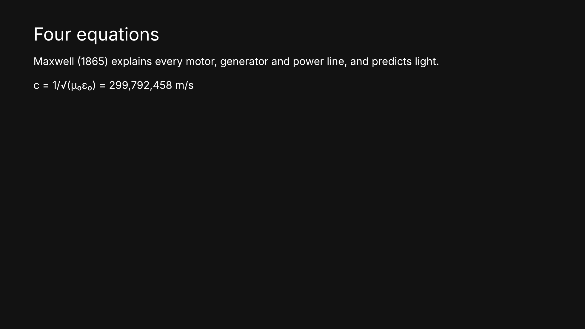
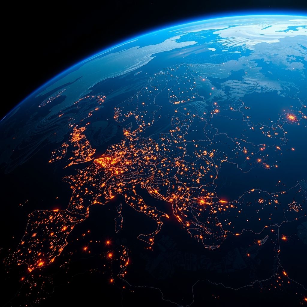
Background: AI-generated (FLUX)In 1865 James Clerk Maxwell wrote four equations. They explain every motor, generator and power line, and they predict light. This chapter uses 16 pieces and 20 tools.
Background: AI-generated (FLUX)KaTeX draws them instantly. An AC wave is just these equations at work (three-phase, drawn inline by function-plot).
Same equations via MathJax: numbered, with hidden MathML for screen readers, and an explorer you can step through with the arrow keys.
Each equation arrives with what it means. Then empty space is assumed, and the wave equation and the speed of light fall out.
SymPy derives the wave equation from Maxwell. SageMath and Maxima re-derive the speed separately. All three agree.
Penrose lays the diagram out from the maths: it is told E ⊥ k and B points out of the page, and solves for a layout that obeys.
A travelling wave in 3D. The electric field (amber) and magnetic field (blue) stay at right angles. Drag to orbit.
PhET's tested simulation, embedded as is.
Maxwell's curl equations stepped on a 360 × 360 grid (the Yee scheme). Rings spread at the speed of light, 30 cm apart at 1 GHz.
for n in range(steps):
Hx[:, :] -= dt / (mu0 * dx) * (Ez[:, 1:] - Ez[:, :-1])
Hy[:, :] += dt / (mu0 * dx) * (Ez[1:, :] - Ez[:-1, :])
Ez[1:-1, 1:-1] += dt / (eps0 * dx) * ((Hy[1:, 1:-1] - Hy[:-1, 1:-1]) - (Hx[1:-1, 1:] - Hx[1:-1, :-1]))
Ez[cx, cy] += np.sin(2 * np.pi * f0 * n * dt) * (1 - np.exp(-(n / 60) ** 2))
Ez *= damp
if n % 3 == 0:The whole simulation is these seven lines: update H from E, then E from H.

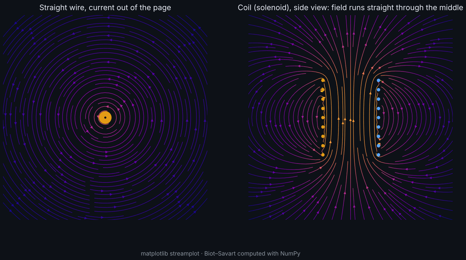
Biot–Savart summed over every bit of wire, then traced with streamplot. A coil straightens the field into a beam through its middle.

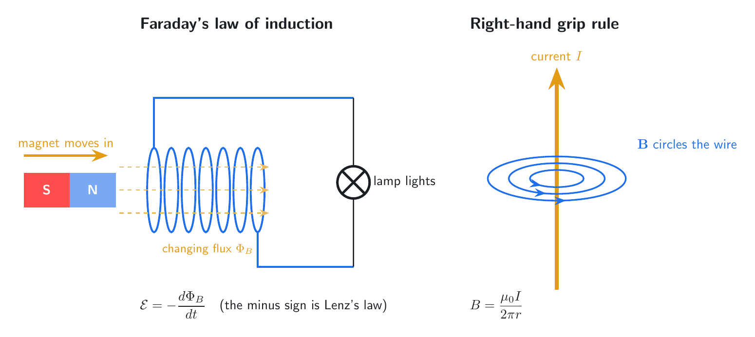
Print-grade figures for the handout: a moving magnet drives current through a lamp, and the grip rule for a wire.
The Lorentz force F = q v × B bends it into a helix. Stepped live in the browser.
Drag the sliders. Real power is V·I·cos φ: shift the current out of phase and the dashed power curve dips below zero.
Rings of arrows circle the current, weaker further out (B ∝ 1/r). Rotate it.
The wave Maxwell predicted: the electric field (amber) and magnetic field (blue) sweep shaded surfaces as the camera flies round. Rendered with OpenGL on the Mac.
Matching an antenna to its feed line on a Smith chart.
Almost every power station spins a magnet inside coils of wire, just as Faraday found. Water, wind, steam and sunlight are just different ways to get there.
Background: AI-generated (FLUX)Fuel burned on the left; electricity made and heat lost on the right. A third to a half of a thermal plant's fuel leaves as waste heat.
How often it runs, what it costs and what it emits. Rotate the cube.
2D physics: falling water pushes the blades round. Click to open the gate wider.
3D physics: gusts push three blades on a hinged hub while the generator holds it back.
A motor turns a solar panel to face the sun from 6 am to 6 pm, simulated with joints and control.

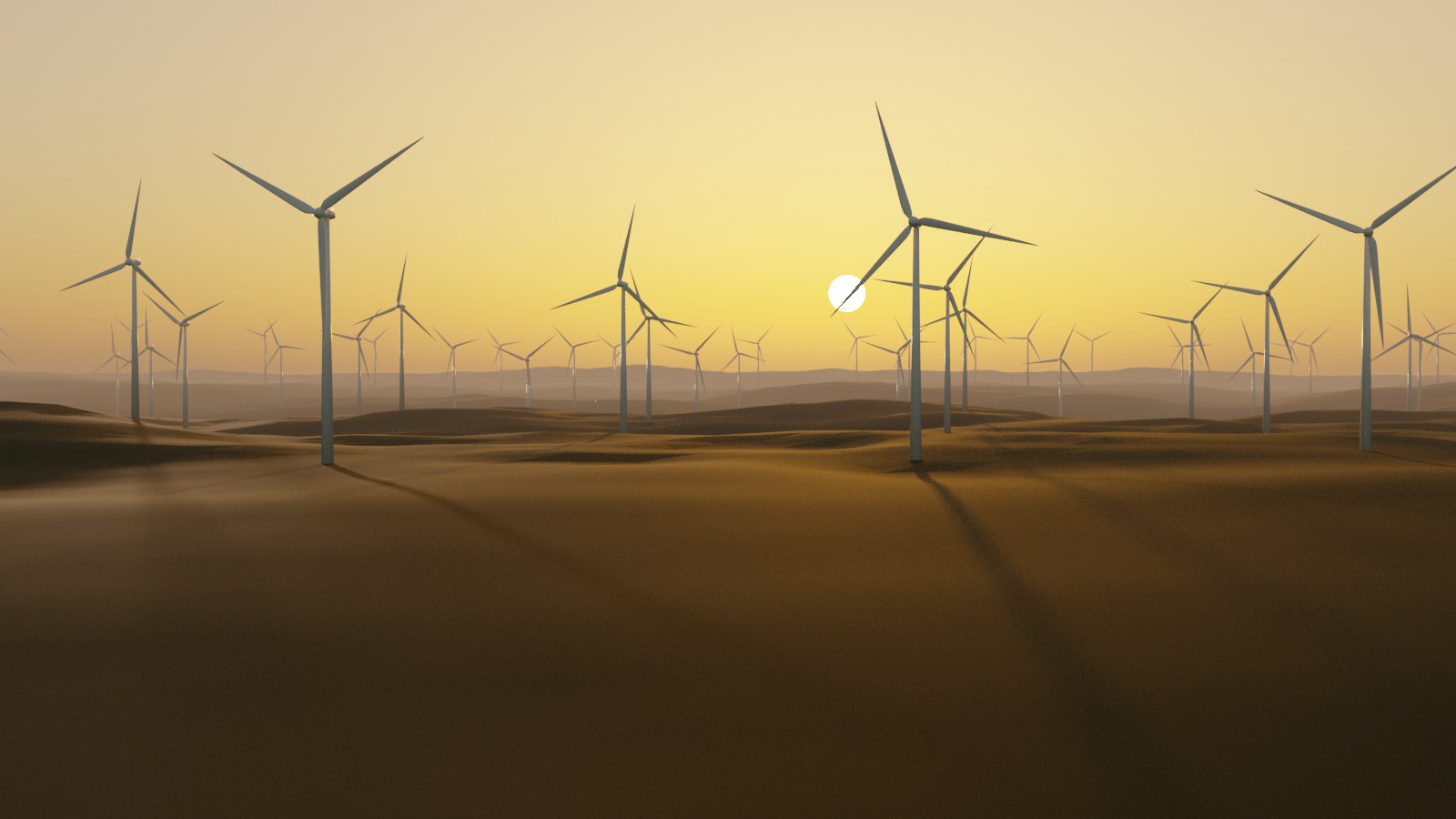
Photoreal rendering, built entirely from code: terrain, sky and 36 turbines.

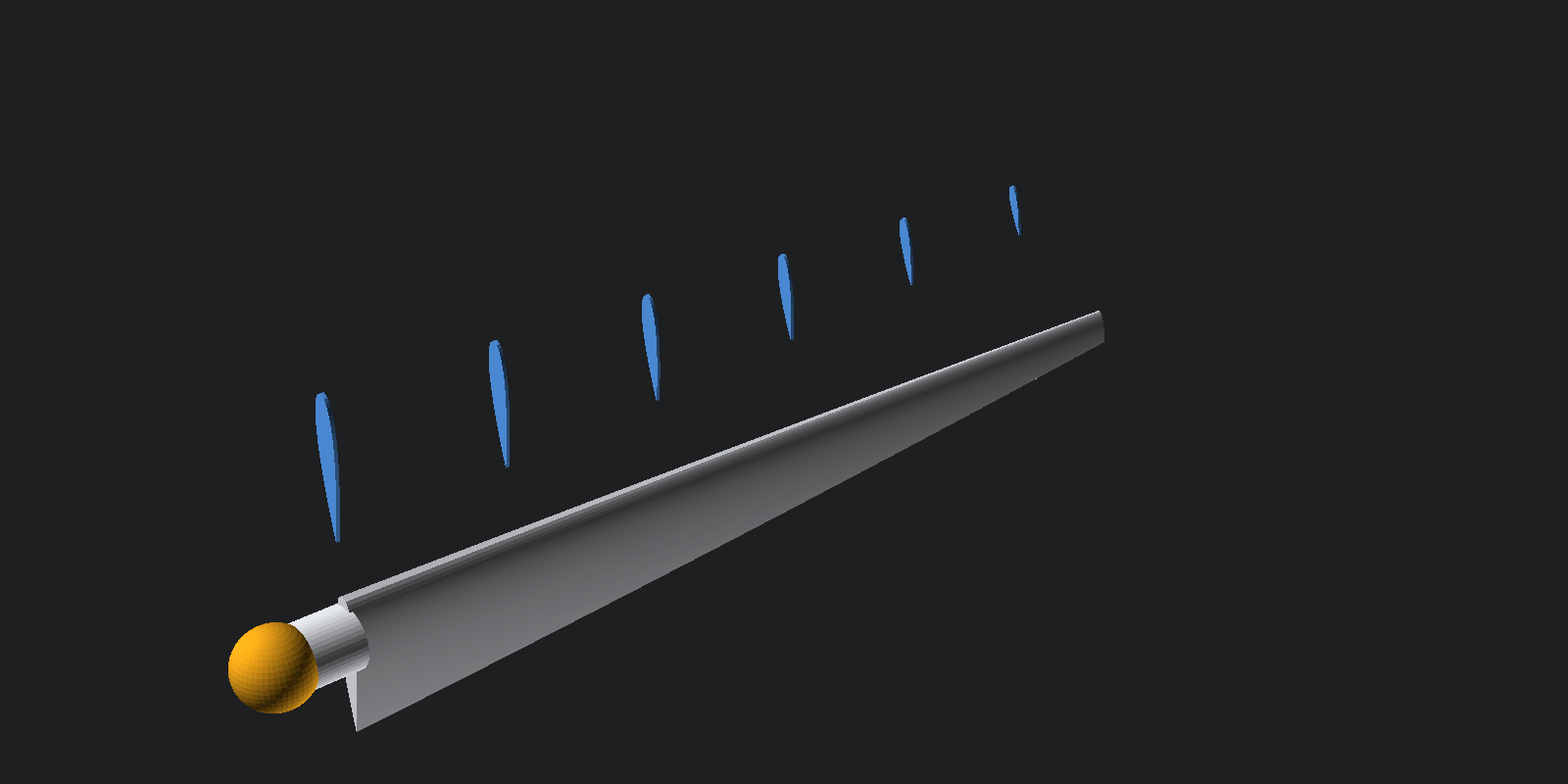
Airfoil sections (blue) show how the blade tapers and twists from root to tip. Change one number; the part rebuilds.
The diamond-lattice crystal every panel is made of, built atom by atom.
Photosystem II, the protein plants use to turn sunlight into electrical charge, loaded live from the Protein Data Bank.
A real photograph where it matters.
An AI cutout turns a flat picture into layers for parallax.
Electricity is made far away and used at 230 V. Transformers, rectifiers and inverters bridge the gap, and the grid keeps everything at 50 Hz.
Background: AI-generated (FLUX)The grid as an architecture diagram. The power lines draw themselves in order: generation, transmission, distribution, home.
Magnetic flux (green) runs round the iron core and reverses with the AC, slowed 100×. The camera follows a keyframed path; grab it to orbit.
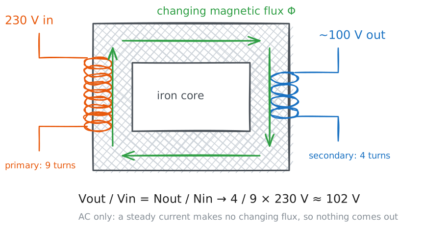
The same idea as a whiteboard sketch: turns ratio sets the voltage, and only AC passes.

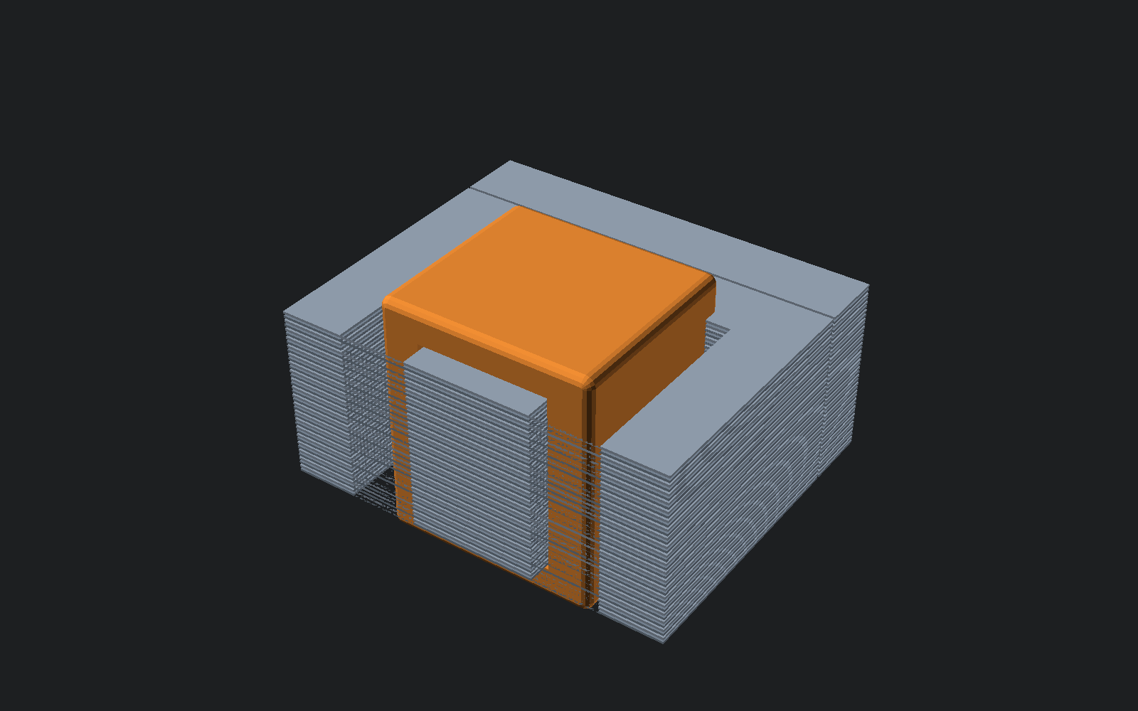
A parametric E-I core: 40 laminations and a copper winding. Change one number in the code and the part rebuilds.
Falstad's simulator: current dots flow through a transformer. Click switches, drag values.
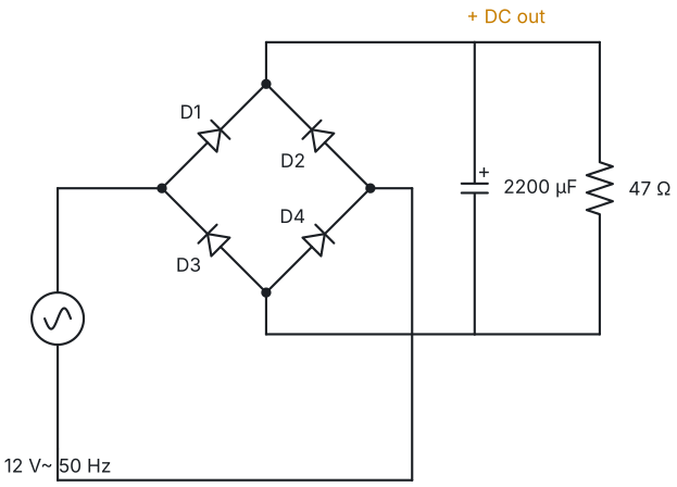
The bridge rectifier in every charger, drawn from code.

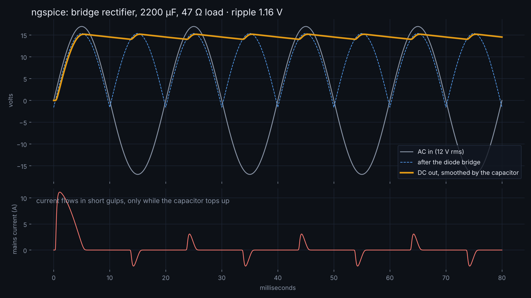
ngspice runs the same circuit. The capacitor holds the voltage up between peaks; the mains current comes in short gulps.
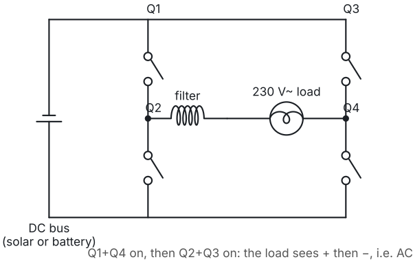
Every solar panel and battery needs one. Four switches flip the load's polarity many times a cycle.
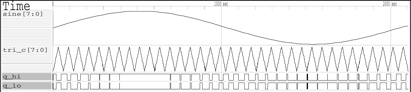
A timing diagram of the H-bridge's gate signals and the voltage the load sees.

The PWM generator written as real Verilog and simulated cycle by cycle. A sine is compared with a fast triangle; the gate signals widen and narrow with the sine.
Drag the current arrow. The angle to the voltage sets how much of the current does real work.
Maxima solves the series RLC filter exactly with a Laplace transform: the voltage rings at 3 kHz and settles in about 5 ms.
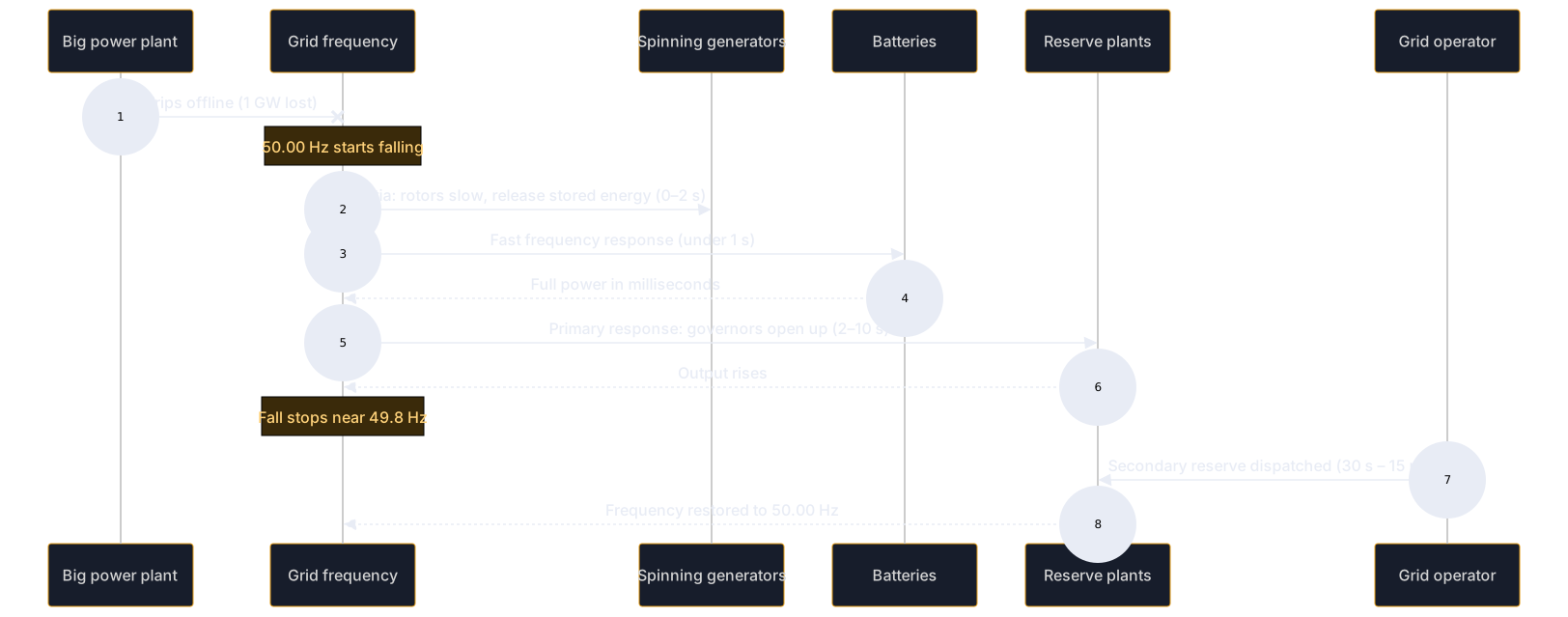
Who reacts, in what order, to hold the grid at 50 Hz.
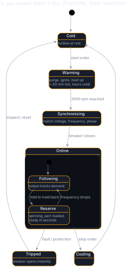
The states a power plant moves through, as a UML state machine.
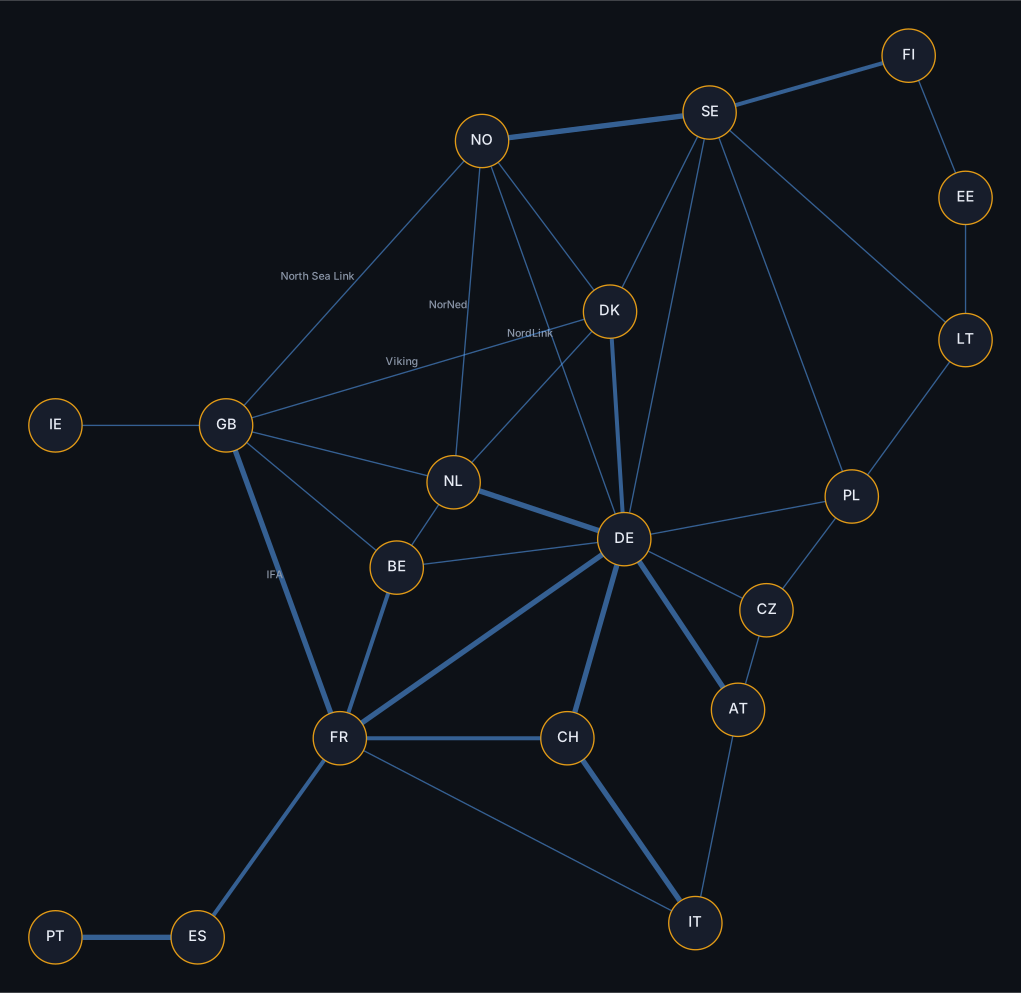
Main cross-border links, laid out automatically. Thicker lines are bigger links.

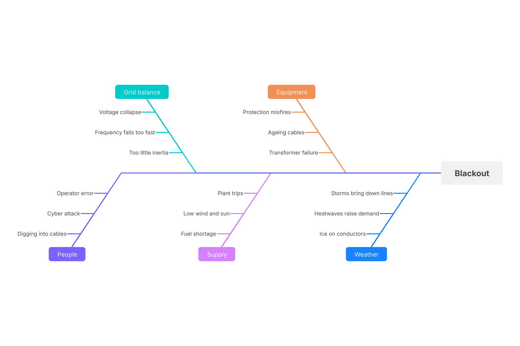
Causes grouped as a fishbone diagram.
The steps as a formal business process (BPMN 2.0), with the branch when the local network is full. Scroll to zoom.
Game-engine rendering. The camera glides until you click; then use WASD or the arrow keys.
A microcontroller counting meter pulses, simulated in the browser.
The same pulse counter as logic gates.
Hundreds of nodes in one transient run.
Stress colours on a transmission tower.
One model, shown at country, region and street level.
With proper IEC electrical symbols.
An open canvas for visitors.
A hover controller fights gravity and gusts while a fan of ray-casts measures the clearance to the conductors. It turns red where the line sags.
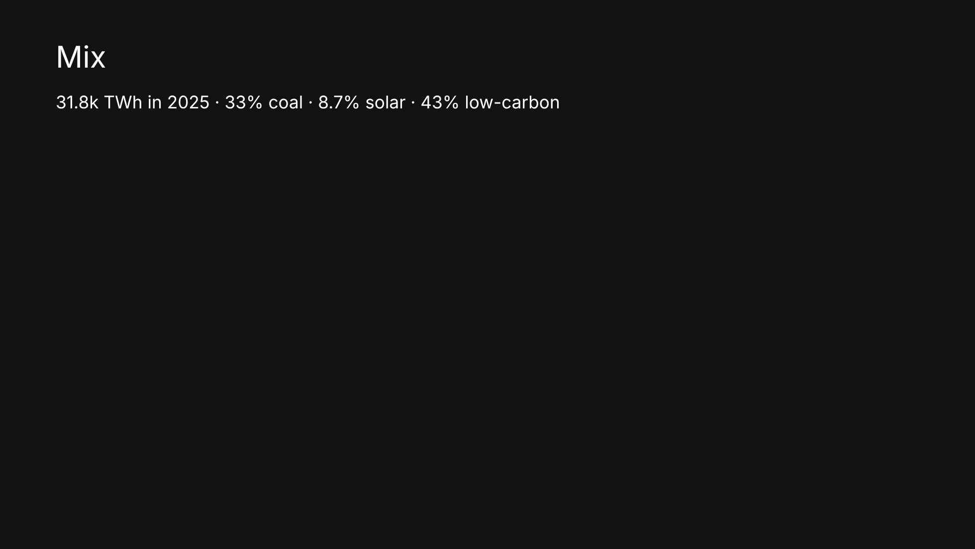
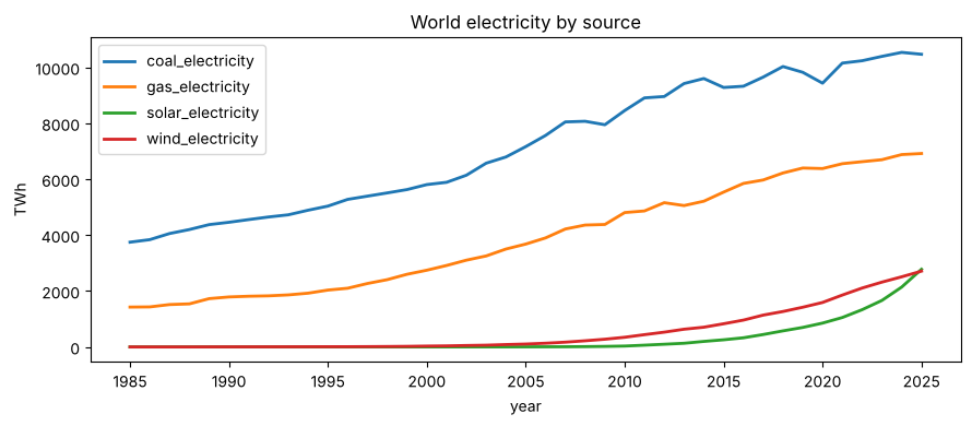
31,772 TWh in 2025. Coal is still the biggest single source; solar is the fastest-growing. Same data, 9 ways.
Background: AI-generated (FLUX)The world's mix re-divides itself year by year while the total climbs. At the end, solar lifts out of the bar.
Each band is a fuel; its width is terawatt-hours that year. Hover anywhere for the numbers.
Coal, gas, solar and wind since 2000. Each panel has its own scale, so small countries are readable too.
Pick a country. A light canvas chart shows its mix for the latest year.
Six races made in bulk from one table, one line of code each.
A recorded terminal session. Pause it and copy any command: it's text, not video.
A scripted terminal clip for the showreel.
Flourish's hosted scrollytelling template, fed the same data.
A newsroom-style, fully responsive chart, made and filled through Datawrapper's API, then published from the Datawrapper account.
Where electricity is clean, and where every one of about 35,000 power plants stands.
Background: AI-generated (FLUX)Low-carbon share of each country's electricity (nuclear plus renewables). Hover a country; the map tours the continents by itself until you touch it.
About 35,000 plants as columns: height is capacity, colour is fuel. Right-drag to tilt and spin; hover a column for its name.
Every plant by start year and size. Big coal and hydro cluster in the past; a swarm of small solar and wind fills the last decade.
A recorded visit to the 12-producers chart, replayed as live page content rather than video, so it stays sharp at any zoom.
A React component rendered frame by frame: the globe's rotation is a pure function of the frame number, so every frame is exact and repeatable.
Sun and wind don't follow demand, so storage matters more each year. Here is what is inside a battery, down to the atoms.
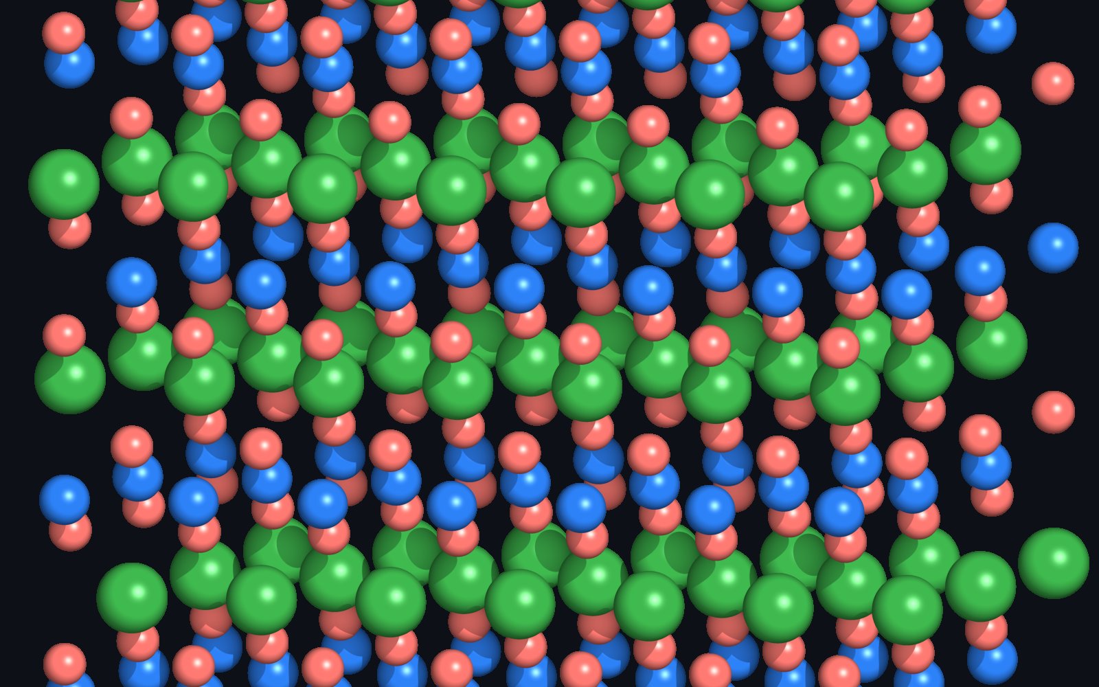
Background: AI-generated (FLUX)Lithium cobalt oxide: lithium (green) sits between layers of cobalt (blue) and oxygen (red). Charging pulls the lithium out. Drag to rotate.

A cover-quality still of the layered structure.
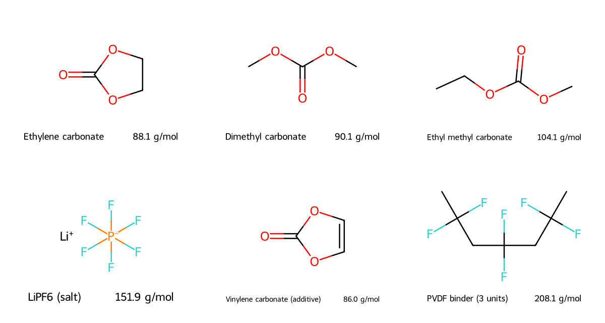
The electrolyte solvents, the lithium salt, an additive and the binder, drawn from their chemical formulas.
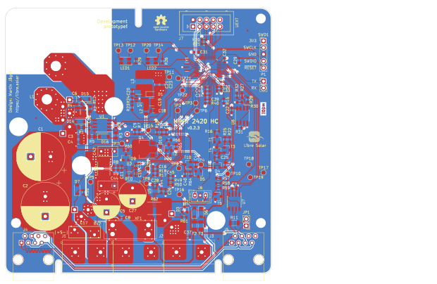
The open-hardware LibreSolar MPPT 2420 HC board, exported straight from its KiCad design files.
The showreel, the talk, the handout and the share card, all made from the pieces above.
Background: AI-generated (FLUX)Five tools' clips cut to a narration, with word-by-word captions and broadcast loudness. The chapter menu came from automatic cut detection.
A multitrack edit with luma transitions between every clip.
Nine tools' output composited into a single moving grid.
A scripted visitor clicks through the page; the video zooms into each click, and the dead time is cut out automatically.
Whisper transcribed the English narration with word timings. It heard Maxwell's middle name as "Kirk"; the captions correct it.
A second voice in a second language.


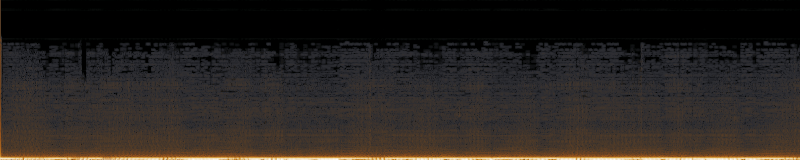
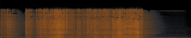
Sound effects generated from a sentence each, with spectrograms (ffmpeg) so you can see them: the hum is one low band, the arc is broadband bursts, the turbine is a slow sweep.


Developer slides from Markdown, with click-by-click reveals.
Nested slides with speaker notes (press S), and a drill-down under Mix (press ↓).
The same story in the formats people ask for.

A notebook recomputes the page's headline numbers from the raw file on every build. nbconvert runs it and pulls out the figures; Quarto publishes it.

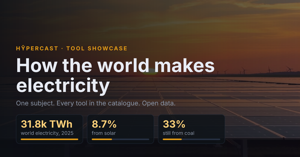
The image shown when this page is shared, laid out in code and rasterised without a browser.

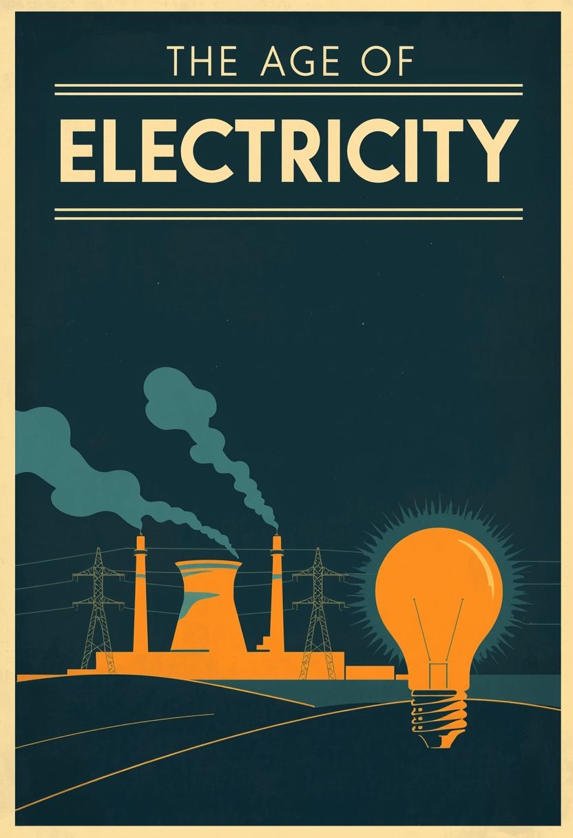
An AI poster with the headline lettered in. The first attempt misspelled it; this is the third.

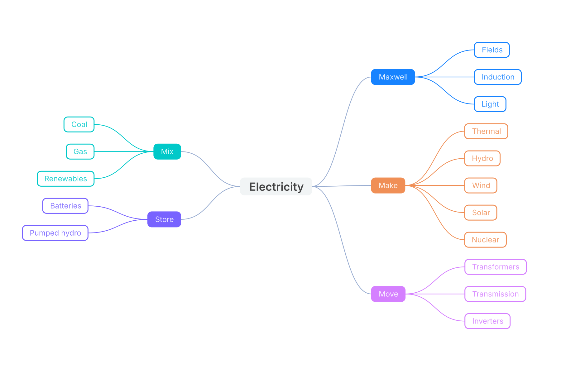
A mind map of the whole page.

Every chapter header image was generated from a text prompt and is labelled as AI-made.
An automatic broadcast check on the showreel. It flags the dark, low-saturation house style: a fair point, and a choice.
An open whiteboard. Add a wind farm, a battery, a rooftop.